《Star Schema Benchmark》阅读笔记

简介

SSB（Star Schema Benchmark）是麻省州立大学波士顿校区的研究人员定义的基于现实商业应用的数据模型，业界公认用来模拟决策支持类应用，比较公正和中立。学术界和工业界普遍采用它来评价决策支持技术方面应用的性能。
SSB 由 TPC（Transaction Processing Performance Council，事务处理性能委员会）发布的 TPC-H 标准改进而来。它将 TPC-H 的雪花模型改为星型模型，将基准查询由 TPC-H 的复杂 Ad-Hoc 查询改为了结构更固定的 OLAP 查询。

事务处理性能委员会（ Transaction Processing Performance Council ），是由数10家会员公司创建的非盈利组织，总部设在美国。该组织对全世界开放，但迄今为止，绝大多数会员都是美、日、西欧的大公司。TPC的成员主要是计算机软硬件厂家，而非计算机用户，它的功能是制定商务应用基准程序（Benchmark）的标准规范、性能和价格度量，并管理测试结果的发布。

引用自百度百科 TPC （事务处理性能委员会）

不使用 TPC-H 的原因是，想要提供更普适的功能覆盖（Functional Coverage）和选择覆盖（Selectivity Coverage）：

功能覆盖（Functional Coverage）：尽可能的选用跨多个表的查询，来贴近实际使用情况
选择覆盖（Selectivity Coverage）：通过维度表的条件来过滤事实表，并使得过滤后的结果集相对较少

几个概念：

SF（Scale Factor）：生成测试数据集时传入的数据量规模因子，决定了各表最终生成的行数。
FF（Filter Factor）：每个 WHERE 过滤条件筛选出一部分行，被筛选出的行数占过滤前行数的比例叫做 FF。在过滤列彼此独立的条件下，表的FF为该表上各个过滤条件FF的乘积。

表结构

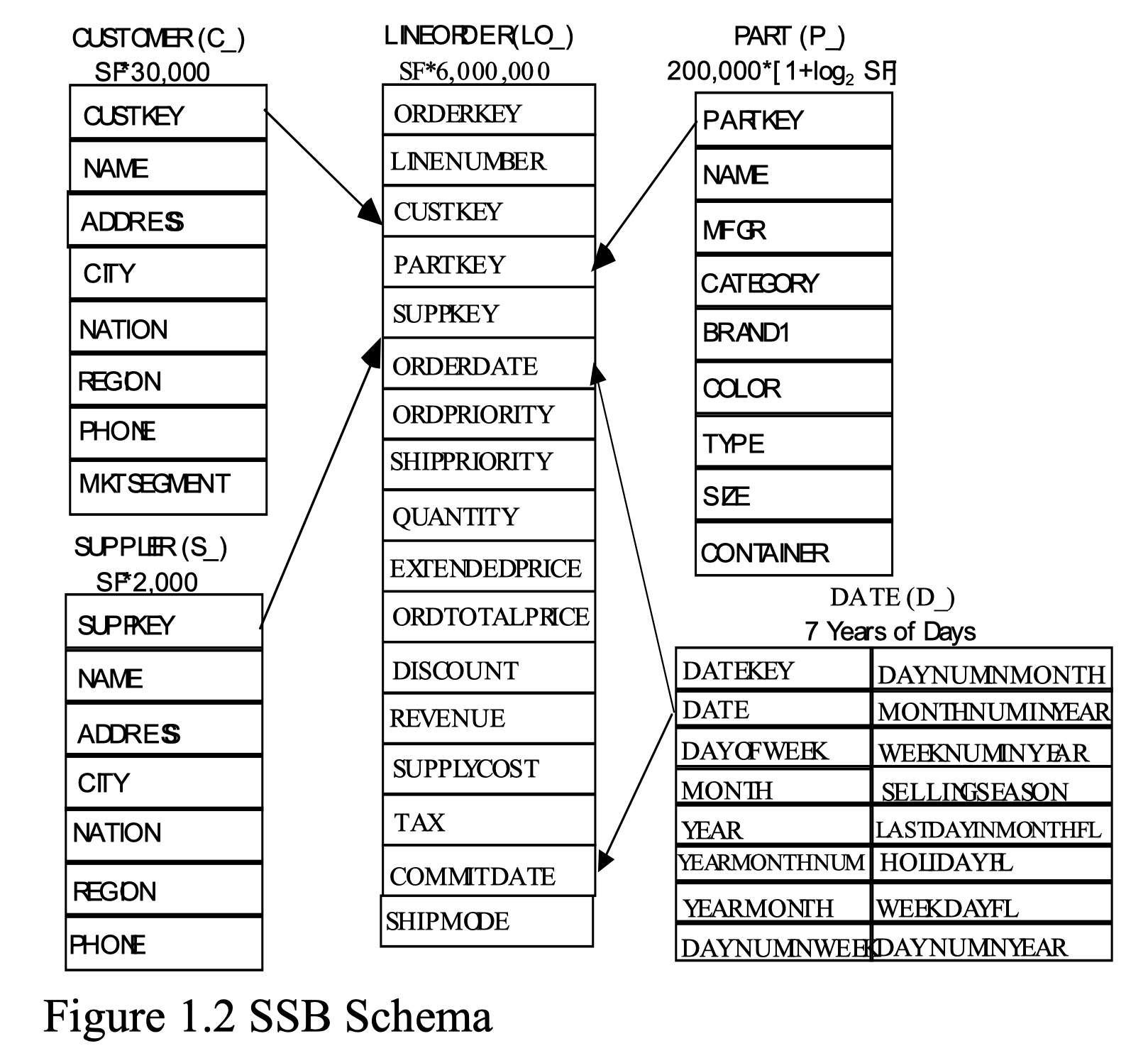
TPC-H 和 SSB 中所有表的规模都从给定的 SF=1 到 SF=10 ，通常表的规模是 SF 的倍数。

LINEORDER 事实表

事实表合并了在 TPC-H 中的 LINEITEM 和 ORDERS 表，更加符合数据仓库的标准，减少了在查询过程中不必要的 join 计算。

规模：$SF*6,000,000$

Schema 描述

字段	描述
LO_ORDERKEY	numeric (int up to SF 300) first 8 of each 32 keys populated
LO_LINENUMBER	numeric 1-7
LO_CUSTKEY	numeric identifier FK to C_CUSTKEY
LO_PARTKEY	identifier FK to P_PARTKEY
LO_SUPPKEY	numeric identifier FK to S_SUPPKEY
LO_ORDERDATE	identifier FK to D_DATEKEY
LO_ORDERPRIORITY	fixed text, size 15
LO_SHIPPRIORITY	fixed text, size 1
LO_QUANTITY	numeric 1-50 (for PART)
LO_EXTENDEDPRICE	numeric ≤ 55,450 (for PART)
LO_ORDTOTALPRICE	numeric ≤ 388,000 (ORDER)
LO_DISCOUNT	numeric 0-10 (for PART, percent)
LO_REVENUE	numeric (for PART: (lo_extendedprice*(100-lo_discnt))/100)
LO_SUPPLYCOST	numeric (for PART)
LO_TAX	numeric 0-8 (for PART)
LO_COMMITDATE	FK to D_DATEKEY
LO_SHIPMODE	fixed text, size 10
Compound Primary Key: LO_ORDERKEY, LO_LINENUMBER

建表 SQL

CREATE TABLE LINEORDER 
(
  LO_ORDERKEY          INTEGER NOT NULL,
  LO_LINENUMBER        INTEGER NOT NULL,
  LO_CUSTKEY           INTEGER NOT NULL,
  LO_PARTKEY           INTEGER NOT NULL,
  LO_SUPPKEY           INTEGER NOT NULL,
  LO_ORDERDATE         INTEGER NOT NULL,
  LO_ORDERPRIORITY     VARCHAR(15) NOT NULL,
  LO_SHIPPRIORITY      VARCHAR(1) NOT NULL,
  LO_QUANTITY          INTEGER NOT NULL,
  LO_EXTENDEDPRICE     INTEGER NOT NULL,
  LO_ORDERTOTALPRICE   INTEGER NOT NULL,
  LO_DISCOUNT          INTEGER NOT NULL,
  LO_REVENUE           INTEGER NOT NULL,
  LO_SUPPLYCOST        INTEGER NOT NULL,
  LO_TAX               INTEGER NOT NULL,
  LO_COMMITDATE        INTEGER NOT NULL,
  LO_SHIPMODE          VARCHAR(10) NOT NULL
);

PART 维度表

规模：$ 200,000*floor(1+log2SF)$

Schema 描述

字段	描述
P_PARTKEY	identifier
P_NAME	variable text, size 22 (Not unique)
P_MFGR	fixed text, size 6 (MFGR#1-5, CARD = 5)
P_CATEGORY	fixed text, size 7 (‘MFGR#’\|\|1-5\|\|1-5: CARD = 25)
P_BRAND1	fixed text, size 9 (P_CATEGORY\|\|1-40: CARD = 1000)
P_COLOR	variable text, size 11 (CARD = 94)
P_TYPE	variable text, size 25 (CARD = 150)
P_SIZE	numeric 1-50 (CARD = 50)
P_CONTAINER	fixed text, size 10 (CARD = 40)
Primary Key: P_PARTKEY

建表 SQL

CREATE TABLE PART 
(
  P_PARTKEY     INTEGER NOT NULL,
  P_NAME        VARCHAR(22) NOT NULL,
  P_MFGR        VARCHAR(6),
  P_CATEGORY    VARCHAR(7) NOT NULL,
  P_BRAND1      VARCHAR(9) NOT NULL,
  P_COLOR       VARCHAR(11) NOT NULL,
  P_TYPE        VARCHAR(25) NOT NULL,
  P_SIZE        INTEGER NOT NULL,
  P_CONTAINER   VARCHAR(10) NOT NULL
);

SUPPLIER 维度表

规模：$SF*2,000$

Schema 描述

字段	描述
S_SUPPKEY	numeric identifier
S_NAME	fixed text, size 25: ‘Supplier’\|\|S_SUPPKEY
S_ADDRESS	variable text, size 25 (city below)
S_CITY	fixed text, size 10 (10/nation:
S_NATION_PREFI	\|\|(0-9)
S_NATION	fixed text, size 15 (25 values, longest UNITED KINGDOM)
S_REGION	fixed text, size 12 (5 values: longest MIDDLE EAST)
S_PHONE	fixed text, size 15 (many values, format: 43-617-354-1222)
Primary Key: S_SUPPKEY

建表 SQL

CREATE TABLE SUPPLIER
(
  S_SUPPKEY   INTEGER NOT NULL,
  S_NAME      VARCHAR(25) NOT NULL,
  S_ADDRESS   VARCHAR(25) NOT NULL,
  S_CITY      VARCHAR(10) NOT NULL,
  S_NATION    VARCHAR(15) NOT NULL,
  S_REGION    VARCHAR(12) NOT NULL,
  S_PHONE     VARCHAR(15) NOT NULL
);

CUSTOMER 维度表

规模：$SF*30,000$

Schema 描述

字段	描述
C_CUSTKEY	numeric identifier
C_NAME	variable text, size 25 ‘Cutomer’\|\|C_CUSTKEY
C_ADDRESS	variable text, size 25 (city below)
C_CITY	fixed text, size 10 (10/nation:
C_NATION_PREFI	\|\|(0-9)
C_NATION	fixed text, size 15 (25 values, longest UNITED KINGDOM)
C_REGION	fixed text, size 12 (5 values: longest MIDDLE EAST)
C_PHONE	fixed text, size 15 (many values, format: 43-617-354-1222)
C_MKTSEGMENT	fixed text, size 10 (longest is AUTOMOBILE)
Primary Key: C_CUSTKEY

建表 SQL

CREATE TABLE CUSTOMER
(
  C_CUSTKEY      INTEGER NOT NULL,
  C_NAME         VARCHAR(25) NOT NULL,
  C_ADDRESS      VARCHAR(25) NOT NULL,
  C_CITY         VARCHAR(10) NOT NULL,
  C_NATION       VARCHAR(15) NOT NULL,
  C_REGION       VARCHAR(12) NOT NULL,
  C_PHONE        VARCHAR(15) NOT NULL,
  C_MKTSEGMENT   VARCHAR(10) NOT NULL
);

DATE 维度表

规模：7 years of days

Schema 描述

字段	描述
D_DATEKEY	identifier, unique id – e.g. 19980327 (what we use)
D_DATE	fixed text, size 18: e.g. December 22, 1998
D_DAYOFWEEK	fixed text, size 8, Sunday..Saturday
D_MONTH	fixed text, size 9: January, …, December
D_YEAR	unique value 1992-1998
D_YEARMONTHNUM	numeric (YYYYMM)
D_YEARMONTH	fixed text, size 7: (e.g.: Mar1998）
D_DAYNUMINWEEK	numeric 1-7
D_DAYNUMINMONTH	numeric 1-31
D_DAYNUMINYEAR	numeric 1-366
D_MONTHNUMINYEAR	numeric 1-12
D_WEEKNUMINYEAR	numeric 1-53
D_SELLINGSEASON	text, size 12 (e.g.: Christmas)
D_LASTDAYINWEEKFL	1 bit
D_LASTDAYINMONTHFL	1 bit
D_HOLIDAYFL	1 bit
D_WEEKDAYFL	1 bit
Primary Key: D_DATEKEY

建表 SQL

CREATE TABLE DATES (
 D_DATEKEY INTEGER,
 D_DATE VARCHAR(18) NOT NULL,
 D_DAYOFWEEK VARCHAR(18) NOT NULL,
 D_MONTH VARCHAR(9) NOT NULL,
 D_YEAR INTEGER NOT NULL,
 D_YEARMONTHNUM INTEGER,
 D_YEARMONTH VARCHAR(7) NOT NULL,
 D_DAYNUMINWEEK INTEGER,
 D_DAYNUMINMONTH INTEGER,
 D_DAYNUMINYEAR INTEGER,
 D_MONTHNUMINYEAR INTEGER,
 D_WEEKNUMINYEAR INTEGER,
 D_SELLINGSEASON VARCHAR(12) NOT NULL,
 D_LASTDAYINWEEKFL INTEGER,
 D_LASTDAYINMONTHFL INTEGER,
 D_HOLIDAYFL INTEGER,
 D_WEEKDAYFL INTEGER
);

查询语句

相对于 TPC-H ，SSB 简化了模型，减少了部分 Table 并增加了新的 Table 。同时在 SQL 上，SSB 在 TPC-H 的基础上，使用尽可能少的 SQL 来得出完整的结论。

查询语句定义

Q1

第一类查询的模板如下

select sum(lo_extendedprice * lo_discount) as revenue
 from lineorder, date
 where lo_orderdate = d_datekey
  and [DATE_FILTER]
  and [LO_DISCOUNT_FILTER]
  and [LO_QUANTITY_FILTER];

其场景是：在一个给定的 时间范围 内，过滤 折扣 和 销售数量 在某个范围内的订单，计算所带来的的 销售收入 之和。

该场景从一个维度表对数据进行限制。

该场景拓展出 3 个查询语句，各个语句过滤出来的数据都没有交集，可以有效避免系统缓存带来的影响（缓存可能会造成后访问的数据没有磁盘 IO 开销）。

Q1.1

为上述变量赋值

1
2
3

DATE_FILTER -> d_year = 1993
LO_DISCOUNT_FILTER -> lo_discount between 1 and 3
LO_QUANTITY_FILTER -> lo_quantity < 25

完整的 SQL 为

select sum(lo_extendedprice*lo_discount) as revenue
 from lineorder, date
 where lo_orderdate = d_datekey
  and d_year = 1993
  and lo_discount between 1 and 3
  and lo_quantity < 25;

其中：$FF = (1/7) * (3/11) * 0.5 = 0.0194805$ ，对于 SF = 1 被过滤出来的 LINEORDER 数量为 $0.0194805 * 6,000,000 ≈ 116,883$。

Q1.2

为上述变量赋值

1
2
3

DATE_FILTER -> d_yearmonthnum = 199401
LO_DISCOUNT_FILTER -> lo_discount between 4 and 6
LO_QUANTITY_FILTER -> lo_quantity between 26 and 35

完整的 SQL 为

select sum(lo_extendedprice*lo_discount) as revenue
 from lineorder, date
 where lo_orderdate = d_datekey
  and d_yearmonthnum = 199401
  and lo_discount between4 and 6
  and lo_quantity between 26 and 35;

其中：$FF = (1/84) * (3/11) * 0.2 = 0.00064935$ ，对于 SF = 1 被过滤出来的 LINEORDER 数量为 $0.00064935 * 6,000,000 ≈ 3896$。

Q1.3

为上述变量赋值

1
2
3

DATE_FILTER -> d_weeknuminyear = 6 and d_year = 1994
LO_DISCOUNT_FILTER -> lo_discount between 5 and 7
LO_QUANTITY_FILTER -> lo_quantity between 26 and 35

完整的 SQL 为

select sum(lo_extendedprice*lo_discount) as revenue
 from lineorder, date
 where lo_orderdate = d_datekey
  and d_weeknuminyear = 6
  and d_year = 1994
  and lo_discount between 5 and 7
  and lo_quantity between 26 and 35;

其中：$FF = (1/364) * (3/11) * 0.1 = 0.000075$，对于 SF = 1 被过滤出来的 LINEORDER 数量为 $0.000075 * 6,000,000 ≈ 450$。

Q2

第二类查询语句的模板如下

select sum(lo_revenue), d_year, p_brand1
 from lineorder, date, part, supplier
 where lo_orderdate = d_datekey
  and lo_partkey = p_partkey
  and lo_suppkey = s_suppkey
  and [PART_FILTER]
  and [S_REGION_FILTER]
 group by d_year, p_brand1
 order by d_year, p_brand1;

其场景是：在给定的 供应商 和 分类 条件下，每个 品牌 每 年 带来的 收入之和。

该场景从两个维度表对数据进行限制。

这个场景也拓展了 3 个查询，这 3 个查询过滤出来的数据互相没有交集，且与 Q1 中的数据没有交集。

Q2.1

为上述变量赋值

1 2	PART_FILTER -> p_category = 'MFGR#12' S_REGION_FILTER -> s_region = 'AMERICA'

完整的 SQL 为

select sum(lo_revenue), d_year, p_brand1
from lineorder, date, part, supplier
 where lo_orderdate = d_datekey
  and lo_partkey = p_partkey
  and lo_suppkey = s_suppkey
  and p_category = 'MFGR#12'
  and s_region = 'AMERICA'
 group by d_year, p_brand1
 order by d_year, p_brand1;

其中：$FF = (1/25) * (1/5) = 1/125$，对于 SF = 1 被过滤出来的 LINEORDER 数量为 $(1/125) * 6,000,000 ≈ 48,000$。

Q2.2

为上述变量赋值

1 2	PART_FILTER -> p_brand1 between 'MFGR#2221' and 'MFGR#2228' S_REGION_FILTER -> s_region = 'ASIA'

完整的 SQL 为

select sum(lo_revenue), d_year, p_brand1
 from lineorder, date, part, supplier
 where lo_orderdate = d_datekey
  and lo_partkey = p_partkey
  and lo_suppkey = s_suppkey
  and p_brand1 between 'MFGR#2221' and 'MFGR#2228'
  and s_region = 'ASIA'
 group by d_year, p_brand1
 order by d_year, p_brand1;

其中：$FF = (1/125) * (1/5) = 1/625$，对于 SF = 1 被过滤出来的 LINEORDER 数量为 $(1/625) * 6,000,000 ≈ 9600$。

Q2.3

为上述变量赋值

1 2	PART_FILTER -> p_brand1 = 'MFGR#2221' S_REGION_FILTER -> s_region = 'EUROPE'

完整的 SQL 为

select sum(lo_revenue), d_year, p_brand1
 from lineorder, date, part, supplier
 where lo_orderdate = d_datekey
  and lo_partkey = p_partkey
  and lo_suppkey = s_suppkey
  and p_brand1 = 'MFGR#2221'
  and s_region = 'EUROPE'
 group by d_year, p_brand1
 order by d_year, p_brand1;

其中：$FF = (1/1000) * (1/5) = 1/5000$，对于 SF = 1 被过滤出来的 LINEORDER 数量为 $(1/5000) * 6,000,000 ≈ 1200$。

Q3

第三类查询语句的模板如下

select c_nation, s_nation, d_year, sum(lo_revenue) as revenue
 from customer, lineorder, supplier, date
 where lo_custkey = c_custkey
  and lo_suppkey = s_suppkey
  and lo_orderdate = d_datekey
  and [CUSTOMOR_FILTER]
  and [SUPPLIER_FILTER]
  and [DATE_FILTER]
 group by c_nation, s_nation, d_year
 order by d_year asc, revenue desc;

其场景是：在给定的 供应商 、客户 和 时间 条件下，求出每个 客户所在国家、供应商所在国家、 每年 的 收入之和。

该场景从三个维度表对数据进行限制。

这个场景拓展了 4 个查询，除了 Q3.3 、Q3.4 之外，其他查询过滤出来的数据互相没有交集，且与 Q1、Q2 中的数据没有交集。

Q3.1

为上述变量赋值

1
2
3

CUSTOMOR_FILTER -> c_region = 'ASIA'
SUPPLIER_FILTER -> s_region = 'ASIA'
DATE_FILTER -> d_year >= 1992 and d_year <= 1997

完整的 SQL 为

select c_nation, s_nation, d_year, sum(lo_revenue) as revenue
 from customer, lineorder, supplier, date
 where lo_custkey = c_custkey
  and lo_suppkey = s_suppkey
  and lo_orderdate = d_datekey
  and c_region = 'ASIA'
  and s_region = 'ASIA'
  and d_year >= 1992 and d_year <= 1997
 group by c_nation, s_nation, d_year
 order by d_year asc, revenue desc;

其中：$FF = (1/5) * (1/5) * (6/7) = 6/175$，对于 SF = 1 被过滤出来的 LINEORDER 数量为 $(6/175) * 6,000,000 ≈ 205,714$。

Q3.2

为上述变量赋值

1
2
3

CUSTOMOR_FILTER -> c_nation = 'UNITED STATES'
SUPPLIER_FILTER -> s_nation = 'UNITED STATES'
DATE_FILTER -> d_year >= 1992 and d_year <= 1997

完整的 SQL 为

select c_city, s_city, d_year, sum(lo_revenue) as revenue
 from customer, lineorder, supplier, date
 where lo_custkey = c_custkey
  and lo_suppkey = s_suppkey
  and lo_orderdate = d_datekey
  and c_nation = 'UNITED STATES'
  and s_nation = 'UNITED STATES'
  and d_year >= 1992 and d_year <= 1997
 group by c_city, s_city, d_year
 order by d_year asc, revenue desc;

其中：$FF = (1/25) * (1/25) * (6/7) = 6/4375$，对于 SF = 1 被过滤出来的 LINEORDER 数量为 $(6/4375) * 6,000,000 ≈ 8,228$。

Q3.3

为上述变量赋值

1
2
3

CUSTOMOR_FILTER -> (c_city='UNITED KI1' or c_city='UNITED KI5')
SUPPLIER_FILTER -> (s_city='UNITED KI1' or s_city='UNITED KI5')
DATE_FILTER -> d_year >= 1992 and d_year <= 1997

完整的 SQL 为

select c_city, s_city, d_year, sum(lo_revenue) as revenue
 from customer, lineorder, supplier, date
 where lo_custkey = c_custkey
  and lo_suppkey = s_suppkey
  and lo_orderdate = d_datekey
  and (c_city='UNITED KI1' or c_city='UNITED KI5')
  and (s_city='UNITED KI1' or s_city='UNITED KI5') 
  and d_year >= 1992 and d_year <= 1997
 group by c_city, s_city, d_year
 order by d_year asc, revenue desc;

其中：$FF = (1/125) * (1/125) * (6/7) = 6/109375$，对于 SF = 1 被过滤出来的 LINEORDER 数量为 $(6/109375) * 6,000,000 ≈ 329$。

Q3.4

为上述变量赋值

1
2
3

CUSTOMOR_FILTER -> (c_city='UNITED KI1' or c_city='UNITED KI5')
SUPPLIER_FILTER -> (s_city='UNITED KI1' or s_city='UNITED KI5')
DATE_FILTER -> d_yearmonth = 'Dec1997'

完整的 SQL 为

select c_city, s_city, d_year, sum(lo_revenue) as revenue
 from customer, lineorder, supplier, date
 where lo_custkey = c_custkey
  and lo_suppkey = s_suppkey
  and lo_orderdate = d_datekey
  and (c_city='UNITED KI1' or c_city='UNITED KI5')
  and (s_city='UNITED KI1' or s_city='UNITED KI5')
  and d_yearmonth = 'Dec1997'
 group by c_city, s_city, d_year
 order by d_year asc, revenue desc;

其中：$FF = (1/125) * (1/125) * (1/84) = 1/1,312,500$，对于 SF = 1 被过滤出来的 LINEORDER 数量为 $(1/1,312,500) * 6,000,000 ≈ 5$。

Q4

第四类查询语句的场景是：在给定的 供应商 、客户 、零件 和 时间 条件下，求出每个 客户所在国家、供应商所在国家、 每年 的 利润之和。该场景从四个维度表对数据进行限制。

Q4 的查询结果与 Q1、Q2、Q3 的结果都是没有交集的，不需要担心 Cache 的影响。但是 Q4.2、Q4.3 的结果都是前一次查询的子集，会受到 Cache 的影响，但是这类查询的流程都会具有这样的特点，不可避免。

Q4.1

select d_year, c_nation, sum(lo_revenue - lo_supplycost) as profit
 from date, customer, supplier, part, lineorder
 where lo_custkey = c_custkey
  and lo_suppkey = s_suppkey
  and lo_partkey = p_partkey
  and lo_orderdate = d_datekey
  and c_region = 'AMERICA'
  and s_region = 'AMERICA'
  and (p_mfgr = 'MFGR#1' or p_mfgr = 'MFGR#2')
 group by d_year, c_nation
 order by d_year, c_nation;

其中：$FF = (1/5) * (1/5) * (2/5) = 2/125$，对于 SF = 1 被过滤出来的 LINEORDER 数量为 $(2/125) * 6,000,000 ≈ 96000$。

Q4.2

假如通过 Q4.1 的结果，我们发现 1997 ~ 1998 年间，利润增加了 40%。此时，我们需要进一步查看这个时间段内导致利润上涨的具体原因，比如通过 s_nation 和 p_category 分组。

Q4 的结果与 Q1、Q2、Q3 的结果没有交集，但是 Q4.2、Q4.3、Q4.4 每个查询都是前一个查询的子集，这依然会收到 Cache 的影响。但是这个场景的分析都会是这个步骤，这不可避免。

于是使用下面的 SQL

select d_year, s_nation, p_category, sum(lo_revenue - lo_supplycost) as profit
 from date, customer, supplier, part, lineorder
 where lo_custkey = c_custkey
  and lo_suppkey = s_suppkey
  and lo_partkey = p_partkey
  and lo_orderdate = d_datekey
  and c_region = 'AMERICA'
  and s_region = 'AMERICA'
  and (d_year = 1997 or d_year = 1998)
  and (p_mfgr = 'MFGR#1' or p_mfgr = 'MFGR#2')
 group by d_year, s_nation, p_category
 order by d_year, s_nation, p_category;

其中：$FF = (1/5) * (1/5) * (2/7) * (2/5) = 4/875$，对于 SF = 1 被过滤出来的 LINEORDER 数量为 $(4/875) * 6,000,000 ≈ 27,428$。

Q4.3

假如通过 Q4.2 的结果，我们发现 1997 ~ 1998 年间大部分的利润增长都是来自 s_nation = 'UNITED STATES' 和 p_category = 'MFGR1#4' 。现在我们想要继续下钻到美国的 城市以及零件的 p_brand1 来看细节。

于是使用下面的 SQL

select d_year, s_city, p_brand1, sum(lo_revenue - lo_supplycost) as profit
 from date, customer, supplier, part, lineorder
 where lo_custkey = c_custkey
  and lo_suppkey = s_suppkey
  and lo_partkey = p_partkey
  and lo_orderdate = d_datekey
  and c_region = 'AMERICA'
  and s_nation = 'UNITED STATES'
  and (d_year = 1997 or d_year = 1998)
  and p_category = 'MFGR#14'
 group by d_year, s_city, p_brand1
 order by d_year, s_city, p_brand1;

其中：$(1/5) * (1/25) * (2/7) * (1/25) = 2/21875$，对于 SF = 1 被过滤出来的 LINEORDER 数量为 $(2/21875) * 6,000,000 ≈ 549$。

查询分析

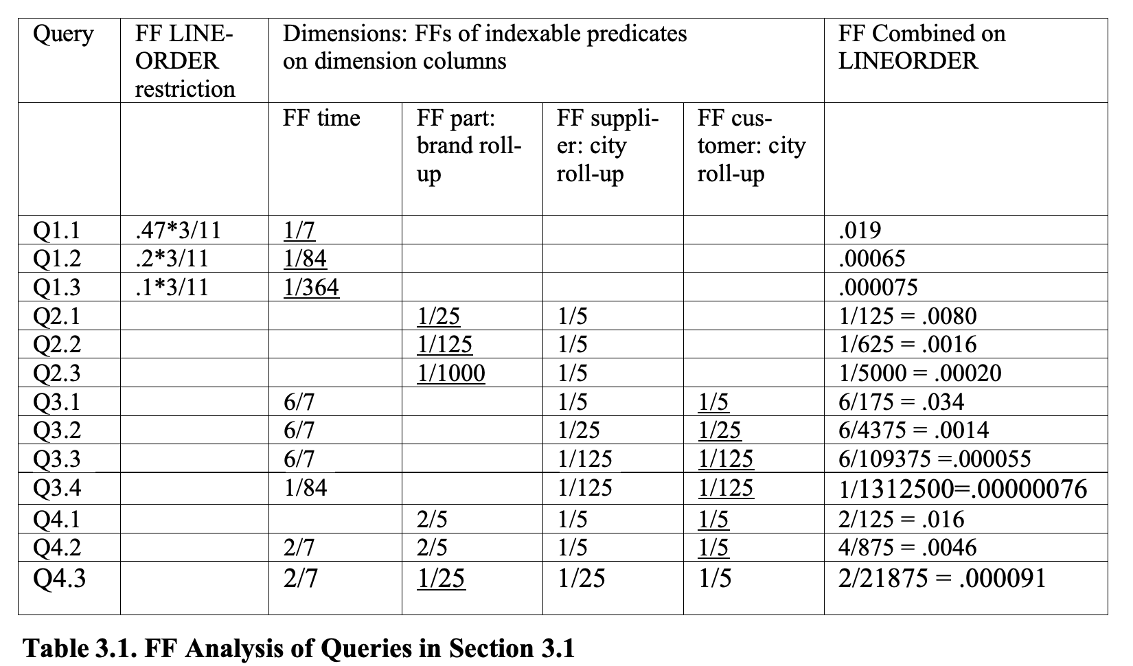
表中带有下划线的 FF 是每个查询中可以被索引的维度列上最小的 FF。加快可被索引的维度列滤列条件的查询的最佳方法是按这一列对 LINEORDER 进行排序，否则可能无法优化磁盘访问。

这一节没怎么看懂，把原文放在这里

The underlined FF for each query distinguishes the smallest FF over the indexable dimension column predicate. The most valuable way we can speed up a query which has an indexable dimension column restriction is to sort the LINEORDER by that column; Otherwise, indexes on such columns will probably not limit the number of disk pages that must be accessed. Note that by breaking ties for underlining away from supplier, we can avoid underlines in the supplier city roll-up column in Table 3.1. Thus we can avoid a LINEORDER sort by s_city. The query set suggests sorts by time, part brand roll-up and (customer roll-up, supplier roll-up).

We see that Q4 shifts from customer-sort to part-sort as best match between Q4.1 and Q4.3.

测试数据

使用 dbgen 可以生成 SSB性能测试的数据，具体方法为

git clone git@github.com:eyalroz/ssb-dbgen.git
cd ssb-dbgen
cmake . && cmake --build .
mkdir data
mv dbgen ./data
cp dists.dss ./data
cd data
./dbgen -v -s 10

工具的一些命令

./dbgen -h
SSB (Star Schema Benchmark) Population Generator (Version 1.0.0)
Copyright Transaction Processing Performance Council 1994 - 2000
USAGE:
dbgen [-{vfFD}] [-O {fhmsv}][-T {pcsdla}]
	[-s <scale>][-C <procs>][-S <step>]
dbgen [-v] [-O {dfhmr}] [-s <scale>] [-U <updates>] [-r <percent>]

-b <s> -- load distributions for <s>
-C <n> -- use <n> processes to generate data
          [Under DOS, must be used with -S]
-D     -- do database load in line
-d <n> -- split deletes between <n> files
-f     -- force. Overwrite existing files
-F     -- generate flat files output
-h     -- display this message
-i <n> -- split inserts between <n> files
-n <s> -- inline load into database <s>
-O d   -- generate SQL syntax for deletes
-O f   -- over-ride default output file names
-O h   -- output files with headers
-O m   -- produce columnar output
-O r   -- generate key ranges for deletes.
-O v   -- Verify data set without generating it.
-q     -- enable QUIET mode
-r <n> -- updates refresh (n/100)% of the
          data set
-s <n> -- set Scale Factor (SF) to  <n>
-S <n> -- build the <n>th step of the data/update set
-T c   -- generate cutomers dimension table ONLY
-T p   -- generate parts dimension table ONLY
-T s   -- generate suppliers dimension table ONLY
-T d   -- generate date dimension table ONLY
-T l   -- generate lineorder fact table ONLY
-U <s> -- generate <s> update sets
-v     -- enable VERBOSE mode

To generate the SF=1 (1GB), validation database population, use:
	dbgen -vfF -s 1

To generate updates for a SF=1 (1GB), use:
	dbgen -v -U 1 -s 1